How Obama Won The Nomination

In early June, Barack Obama clinched the Democratic Party’s nomination for president, besting Hillary Clinton in the most amazing primary battle in the contemporary era. The immediate cause of Clinton ’s departure from the race was probably Obama’s lead in pledged delegates — which, by the end of the primary season, stood at a small-but-significant 106, out of 3,406 total pledged delegates.¹  It was simply impractical for Clinton to count on the so-called “superdelegates” to close the gap between the two.

Meanwhile, Obama’s lead in the actual vote count was vanishingly small, just 150,000 votes out of 35 million cast for the two, without Michigan having fully participated. Thus, by the end of the primaries, Obama had amassed a 3.1 percent lead in pledged delegates, compared to a 0.4 percent lead in votes. This implies that Obama’s voters were more efficient than Clinton’s voters at producing delegates. Indeed, for every Obama delegate, there were 10,788 Obama supporters. For every Clinton delegate, there were 11,727 Clinton supporters.

This efficiency advantage probably made the difference for the junior senator from Illinois. If Clinton ’s voters had been as efficient at producing delegates as Obama’s voters, his lead in pledged delegates would have shrunk from 106 to a paltry 14, which would have placed Clinton well within striking distance of the nomination. Thus, it behooves us to ask how it was that Obama supporters produced more delegates.

This essay will argue that Obama was favored by the delegate allocation system. In other words, Obama won not simply because he had more supporters, but also because the “rules of the game” made those supporters better at generating delegates. To see how this occurred, we will first review the voting coalitions that Obama and Clinton forged over the course of their five-month primary battle. Then, we will investigate the rules of the delegate allocation process to see how they translated each candidate ’s votes into delegates. First, though, comes some theoretical background — a frame of reference for understanding the importance of the rules of delegate allocation. The puzzle that we are faced with relates to a general subject matter that social scientists refer to as “social choice.”

Processing preferences

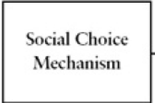
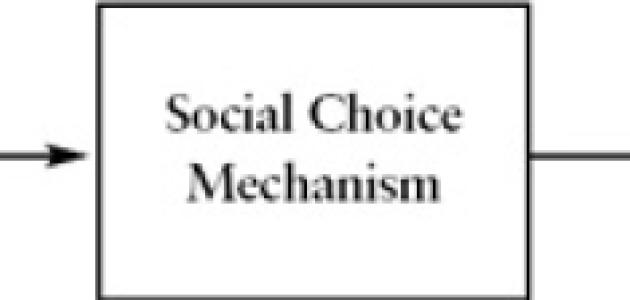
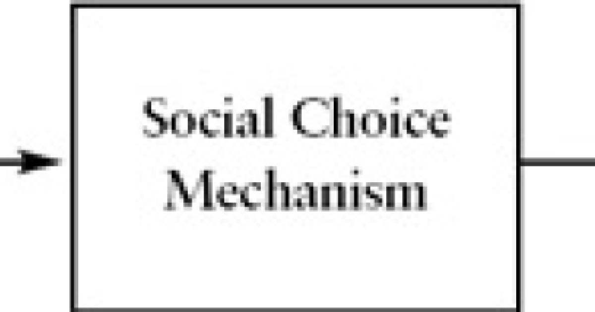
The democrats’ delegate system is designed to aggregate the individual preferences of primary and caucus voters into the choice of the party as a whole, or a social choice. Voters vote; delegates are selected according to those votes; those delegates select a nominee at the party ’s convention. Thus, the nomination process can be understood as a social choice mechanism that translates the preferences of Democrats nationwide into an outcome.

Generally, we might think of it in this way:

We should not assume that the middle step, where individual preferences are processed by the social choice mechanism, is a purely efficient one. Indeed, following Arrow ’s Theorem, we cannot make such an assumption. No social choice mechanism is always able to satisfy even a basic set of normative criteria. In other words, there is no “perfect” voting system. Every conceivable system has ways that the particular rules can influence the outcome, depending upon how preferences are arranged.

Thus, it is often profitable to evaluate the rules of a social choice mechanism to see how they have influenced the outcome. We shall do that for the Democratic nomination process, which is a social choice mechanism like any other. It takes the preferences of individual Democrats and translates them into a choice of all Democrats.

Our argument will be that the particular rules of the process were very important in determining the party ’s nominee, that there were features of the system that favored Obama over Clinton, and that slight, uncontroversial changes in the rules could have produced a different outcome. If we were to compare the nomination process to a translator acting as an intermediary for two conversants who speak different languages, we would be arguing that the translator himself influenced the course of the conversation. Change the translator and you change the conversation.

This intuition can perhaps be understood by reflecting upon the Electoral College. The country as a whole votes for president of the United States. However, the votes are counted per state, with every state being issued a certain number of electors who then cast a second vote at the Electoral College. Thus, the preferences of individual citizens are aggregated into a national choice via the Electoral College. This process can occasionally have an effect on the outcome. The 2000 election is a case in point. The outcome was determined not simply by who had more votes, but also the rules for how those votes were to be counted. More citizens voted for Al Gore than for George W. Bush. However, because Bush ’s voters were distributed in a certain way, the Electoral College awarded him the presidency.

We shall undertake a similar review of the Democratic nomination process which, it must be said, does not have the same kind of intentionality behind it. Whatever one wishes to say about the Electoral College, one cannot argue that its effects were unintended. The Framers gave many reasons for designing it the way they did. For arguments in favor of the utility of the Electoral College, one need simply consult Federalist 68.

In contrast, the Democratic nomination process is a hodge-podge that lacks an internal logic. Its origins trace to the tumultuous 1968 convention. Meeting in Chicago, party bosses awarded the nomination to Vice President Hubert Humphrey, despite the fact that he had participated in no primaries. The resulting turmoil ultimately induced the party to adopt a series of reforms requiring that state parties open their delegate selection processes to the party electorate at large. Eventually, this produced the primaries and caucuses the Democrats now have.

At its core, then, the Democratic system is a hybrid that straddles two distinct political cultures. The quadrennial convention, which has its roots in the political milieu of the nineteenth century, remains to this day. So also does the idea of selecting delegates to vote at the convention. These are decidedly old procedures that the reformers did not eliminate. Instead, they grafted onto them a series of twentieth-century innovations.

And so, part of the nomination process is contemporary; part of it is antiquated. There is no underlying rationality to it. Unfortunately, the Democratic Party has spent very little effort over the years improving it. There was a collective will to reform the system in the early 1970s, but since then little has been done to it.

Voting coalitions

The rudimentary flowchart offered above serves as an analytical roadmap for our work. We are interested in how the rules of the Democratic nomination helped produce the nominee that was produced. This requires us to have an understanding of who voted for each candidate — the voting coalitions that each candidate forged.

Interestingly, each candidate’s voting coalition seems to have been quite stable over the course of the primary campaign. There was hardly any evidence of “momentum” at all. Thus, time effects play only a modest role, and we can understand the results of the New Hampshire primary (held January 8) and South Dakota primary (held June 3) without worrying about how time influenced the vote. The only exception to this general rule is a modest one — the African American vote trended towards Obama over time. At the beginning of the race, in South Carolina, for instance, Hillary Clinton was able to garner around 20 percent of African Americans. Toward the end, in North Carolina, for instance, her numbers were down to below 10 percent.

Let’s begin by examining how Obama and Clinton performed in geographical regions across the country, making use of the Census Bureau ’s definitions. First, let us examine the regions east of the Mississippi River (Figure  1).

As we can see, there are some interesting variations by region. In New England, Clinton scored an 8-point victory overall, owing largely to her victory in Massachusetts. She also swept him in the three Mid-Atlantic states — New York, Pennsylvania, New Jersey.

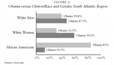
The South Atlantic region is where Obama posted his largest victory of all, and it is worth commenting upon in some detail. Let ’s break the region down by race, and then by gender among whites (Figure 2).

The racial gap in the South was very pronounced. These numbers produced such a large Obama victory because African Americans constituted almost one out of every three voters in the region. Because they broke so heavily to Obama, he was able to win handily.

Let’s return to Figure 1. The “South Central” region — consisting of Tennessee, Kentucky, Mississippi, and Alabama — behaved similarly to the South Atlantic. Clinton won the South Central because there were fewer African Americans who participated there. The “North Central” region — consisting of Ohio, Indiana, Michigan, Illinois, and Wisconsin — is interesting for its internal variation. While overall, the region sported a modest Obama victory, in fact there was a split within it. Clinton won three states — Indiana, Michigan (which we count by allocating all of the “Undeclared” vote to Obama), and Ohio. These wins were more than balanced by Obama’s landslide victories in Illinois and Wisconsin.

What about west of the Mississippi?

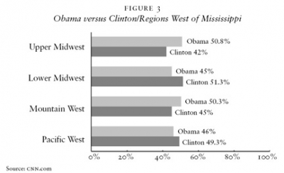
Generally speaking, Obama performed better west of the Mississippi than he did east of it (Figure 3). Beginning with the upper Midwest, we see a 9-point Obama victory, powered in large part by his caucus state wins. There were two primaries in the region — South Dakota, which Clinton won comfortably, and Missouri, which Obama won barely. The lower Midwest went for Clinton in large measure because of Texas. She also won Arkansas and Oklahoma, while he won Louisiana.

Obama’s five-point victory in the Mountain West is a product of a split within the region. Clinton won the states in the south, New Mexico and Arizona, while Obama won the states in the north, Idaho, Montana, and Wyoming. They split the states in the middle of the region, with Obama winning Colorado and Utah and Clinton winning Nevada. Finally, Obama won every state in the Pacific West by comfortable margins except California, which is why Clinton carried the region.

During the primary season, there was frequent commentary upon the demographic groups that Clinton and Obama were winning. Typically, Obama won “upscale” white voters (i.e. those with college degrees and/or incomes greater than $75,000) and African Americans. Clinton won “downscale” white voters and Hispanics. By and large, this narrative was accurate — though there were a few exceptions. In the Mountain West and the Pacific West, Obama was able to win a fair portion of “downscale” white voters. In the Northeast and Mid-Atlantic regions, Clinton was able to perform well with “upscale” whites.

Because we are interested in how these voting coalitions helped produce the political outcome they did, it is worthwhile to analyze these primary results according to political characteristics. Let ’s begin by categorizing the states according to their behavior in past presidential elections. We ’ll develop four categories. “Safe Democratic” states are those that voted for Bill Clinton in 1996 and gave John Kerry a victory of more than 5 percent in 2004. “Lean Democratic” states are those that voted for Clinton and gave Kerry a victory of less than 5 percent. “Lean Republican” states are those that voted for Clinton and gave George W. Bush a victory in 2004. Finally, “Safe Republican” states are those that voted for Bob Dole in 1996 and Bush.

The results are intriguing (Figure 4). Obama and Clinton essentially split the Democratic states. Obama enjoyed a small victory in all safe Democratic states, though he actually won nine of the 14 states in this category. In “lean Democratic” states, Obama’s lead in the overall vote was a little larger, though still not very large. What is more, each candidate won three of the six states. In “lean Republican” states, Clinton trounced Obama by nearly 13 points, winning 11 out of the 13 states in this category. Obama returned the favor in safe Republican states, winning by 11 points and carrying 15 of the 19 states in this category.

Another political category of importance is the type of contest. Pledged delegates were selected either by primaries or by caucuses. As Figure 5 makes clear, each candidate’s performance was strongly correlated to the type of contest.

This, too, is intriguing. Clinton actually won a bare plurality of the vote in the 38 states that held primaries. She and Obama split those states, both winning 19 apiece. The caucuses, however, produced an extremely lopsided result. Obama defeated Clinton on the order of 2–1 in the caucus states, winning all but one of them.

Interestingly, the type of contest might have had a causal effect on Obama’s performance. That is, if the contests had been primaries rather than caucuses, Obama ’s vote share might have declined. Washington state, Nebraska, and Idaho allocated their delegates by the results of their caucuses. At some point afterwards, each held nonbinding primaries, or beauty contests. In the caucuses, Obama defeated Clinton in Washington and Nebraska by 2–1, and by 4–1 in Idaho. In the nonbinding beauty contests, Obama’s margins fell to just five points in Washington, two points in Nebraska, and 18 points in Idaho. Meanwhile, Texas was the only state to allocate delegates by primary and caucus. Both contests were held on the same day. Clinton won the Texas primary by four points. However, Obama bested Clinton in the caucuses by 12 points. That’s a 16-point swing on the same day.

These differing results might have been a consequence of the enthusiasm gap that separated the two candidates. That is, Obama supporters were much more willing than Clinton supporters to participate in the caucus process, which can be time-consuming. These results might also have been induced by the difference in socioeconomic status between each candidate ’s voting coalition. Upscale white voters were more likely to support Obama, and they might have had more time to participate in caucuses. Downscale whites were more likely to support Clinton, and they might have had a harder time sacrificing two hours or more to participate.

The delegate allocation process

How did these voting coalitions produce the delegates for each candidate? This requires us to examine the delegate allocation process. As we indicated earlier, it is this process that translated votes into delegates. Our interest is in this act of translation, and what kind of effect it had on the final result. What we find is that the allocation system has biases or predispositions in its translation of votes into delegates. This is meant in a morally neutral sense. The delegate allocation system is prone to award candidates the more they win voters of a certain type.²

We can detect these biases by deductive and inferential means. The allocation of delegates to states flows ultimately from a fairly straightforward mathematical formula. We can deduce potential biases from the formula, and check those deductions against the actual allocation of delegates. The formula, or “allocation factor,” by which delegates are allocated to states and the District of Columbia is defined thusly:

Allocation Factor = 1⁄2 × ((sdv ÷ tdv) + (sev ÷ 538))

Where:

• sdv is a state’s Democratic vote for president from 1996 through 2004.
• tdv is the total Democratic vote for president across all states from 1996 through 2004.
• sev is the state’s electoral votes as of 2004.

The allocation factor is thus a simple arithmetic mean. It averages a state’s contribution to the Democratic Party’s presidential vote against its contribution to the Electoral College, and therefore its population. So, it weighs Democratic partisanship against population.

This formula produces at least three biases that favored Barack Obama: the small-state bias, the Republican-state bias, and the caucus-state bias.

The small-state and Republican-state biases. Let’s begin with the small-state bias. Because the Electoral College is used as a metric for population, the allocation formula should inherit the small state bias of the Electoral College, which derives from two sources.

(a) Because no state can have fewer than three electors, states with small populations will have more electors per person than states with large populations. For instance, in 2004 Wyoming had three electors and an estimated population of 510,000, for a total of 170,000 people per elector. California had 55 electors and an estimated population of 35.89 million people, for a total of 652,545 people per elector.

(b) Because electors have to be distributed across 50 states and the District of Columbia, rounding is necessary. Some states with unequal sizes will nevertheless receive an equal number of electors. For instance, in 2004 New Hampshire had four electors and an estimated population of 1.30 million, for a total of 325,000 people per elector. Rhode Island had four electors and a population of 1.08 million, for a total of 270,000 people per elector. In other words, Rhode Island was better represented in the Electoral College in 2004 because it was smaller.

Because the allocation factor uses the Electoral College as its metric for population, it retains this bias. Democratic primary voters in small states will be better represented at the Democratic National Convention in Denver because they live in small states.

We can confirm the presence of this effect graphically via the following Charts. The x-axis tracks the voting population by measuring the number of voters per state who voted Democrat or Republican in 2004. The y-axis tracks how well represented each state is at the Democratic convention. It divides a state ’s number of 2004 Kerry voters (a rough measure of Democrats per state) by its number of pledged delegates. The idea is that the fewer Kerry voters per pledged delegate, the better represented state Democrats are at the convention.

If the small-state bias is in effect, we should find small states in the bottom-left and large states in the top-right. Indeed, this is what we find. Interestingly, the relationship is nonlinear. When a state is small, small increases in the size of its electorate dramatically reduce the extent to which the state ’s Democrats are represented at the convention. When a state is very large, it takes very large increases in population to reduce the state ’s representation even a little bit.

We can get a better look at this data array if we “linearize” it by taking the natural log of the total two-party vote (Chart 2). This will have the effect of transforming the pattern into a straight line without altering the underlying trend.

This makes matters much more clear. As we can see, the small states cluster in the lower-left and the large states are in the upper-right. Note, however, that Texas does not fit the pattern very well. If we take a closer look at the graph, we can see a general pattern of which Texas is only the most obvious part. For a given population size, Democrats in Republican states seem to have better representation than Democrats in swing or Democratic states.

This pattern is not illusory. Recall that the allocation factor is simply the average of a state ’s Democratic partisanship and its population. This has the effect of favoring Democrats who live in Republican states. A state that disproportionately favors Republicans will have a smaller contribution to the Democratic vote than to the Electoral College. Thus, averaging the Democratic vote with the share of the Electoral College will make the allocation factor larger for Republican states. Meanwhile, states that disproportionately favor Democrats will have a greater contribution to the Democratic vote than the Electoral College. Thus, averaging the Democratic vote with the Electoral College will make the allocation factor smaller for Democratic states. This is the source of the Republican state bias.

We can appreciate this via an example. Let’s look at Indiana, Missouri, Tennessee, and Washington (Figure 6) — all of which have the same number of Electoral College votes (11).

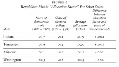
Note that Indiana, which voted Republican in the last three elections, receives a boost while Washington, which has voted Democratic in the last three elections, receives a burden. Missouri, which has voted more Democratic than Tennessee in the last three elections, also receives a burden.

Chart 3 demonstrates the generality of this pattern. The y-axis retains our metric for representativeness. The x-axis measures George W. Bush ’s share of the two-party vote in the last presidential election, our metric to gauge a state ’s Republican tilt.

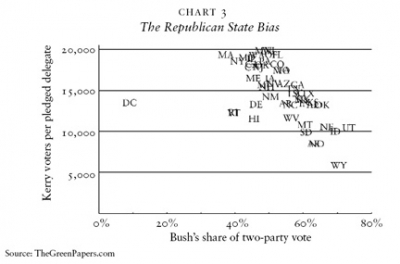
Of course, there is evidence of the small-state bias here. Smaller states tend to be in the bottom-right, and larger-states in the top-left. Nevertheless, the tight band of observations that go from the top-left to the bottom-right as Bush ’s share of the vote increases demonstrates this Republican bias very clearly. A few examples can amplify this point.

(a) Maine, Idaho, and New Hampshire. All have roughly equal populations. Maine, a consistently Democratic state, is in the top-left and Idaho, a consistently Republican state, is in the bottom-right. New Hampshire, a swing state, falls between the two.

(b) Texas and Illinois. If there were just a small-state bias, Illinois Democrats should be better represented than Texas Democrats. After all, Illinois is smaller than Texas. In fact, the opposite is true. Texas Democrats are better represented.

(c) Alabama and Connecticut. We see the same relationship. Connecticut is smaller, but Alabama Democrats are better represented.

What kind of effect did the small-state and Republican-state biases have on the Democratic nomination? Combined, they created a modest, pro-Obama movement in delegate allocation. If we “correct” for these biases by allocating delegates strictly according to each state’s share of the Democratic vote, we would find that Obama’s lead in pledged delegates would have decreased by about 25 percent, from 106 to 80.

This should not come as a surprise. Obama tended to win smaller states, while Clinton won larger states. What is more, as the previous section made clear, Obama had an enormous advantage in the Republican states.

The caucus-state bias

Of the small-state and Republican-state biases exist because of what is included in the allocation factor, the caucus-state bias exists because of what is excluded. That is, the allocation factor does not account for actual participation of statewide Democrats. Thus, Democrats who participate in a low-turnout state have greater influence on the convention than Democrats who participate in a high-turnout state.

Taking only the states that held primaries, this bias would be fairly inconsequential and would probably not break in one direction or the other. The reason is that turnout was generally high across primaries — though it dipped a bit on Super Tuesday. Thus, if we were to adjust the allocation factor to account for differences in primary turnout, we would find no significant boost for either candidate.

What did have an effect, one greatly beneficial to Obama, was the fact that turnout in caucus states was much lower than turnout in primary states. In the caucus states, turnout averaged just 16 percent of Kerry’s 2004 vote. Compare that to the average of 73 percent turnout in the primaries, and we can begin to understand Obama’s advantage. Because the delegate allocation factor does not take turnout into account, his caucus supporters were thus worth many more delegates than they would have been had there been higher turnout. Across all caucuses, Obama won about 679,000 supporters and 280 delegates. Clinton won about 379,000 caucus supporters and 145 delegates. Thus, for a net of 300,000votes, Obama netted 135 delegates. To put this into perspective, consider that Clinton defeated Obama by more than 500,000 votes in California, but only netted 38 delegates.

Unlike the small-state and Republican-state biases, we cannot estimate precisely how including turnout in the allocation factor would have changed the number of delegates each candidate won. After all, the effect would depend upon how we choose to incorporate turnout in the factor. What we can say is that any inclusion of turnout would have aided Clinton. Obama enjoyed a huge advantage in the caucus states because turnout was not determinative in allocating delegates.

One alteration that might have had a dramatic effect would have been turning the caucuses into primaries. It is not simply that turnout in the caucuses was lower than the primaries; it is also that a caucus electorate and primary electorate in the same state might have had very different preferences. We noted earlier that the results in the Washington state, Nebraska, Idaho, and Texas caucuses differed dramatically from the primary results in each state. From the caucuses to the nonbinding primaries, Obama ’s margin of victory dropped on average 30 points, from 36 percent to just 6 percent. If every caucus state had held a primary instead, and Obama’s delegate margin had dropped by 30 points in each, he would have netted fewer than 10 delegates from the caucuses. Obviously, we cannot conclude that this is what would have happened. Instead, the point here is simply that Obama received a very great benefit from these low-turnout caucuses.

Rules matter

This essay has endeavored to accomplish several tasks. First, noting that Obama’s lead among pledged delegates was significantly larger than his lead in the popular vote, it asked how that might have occurred. It then went on to offer a theoretical frame for understanding the question, then a general outline of Obama and Clinton ’s voting coalitions. From this, it showed that the delegate allocation system favored Obama ’s voting coalition in several important ways. This is how he was able to enhance his delegate lead relative to his vote lead.

The implication of this argument is not that Hillary Clinton somehow should have been the Democratic Party ’s nominee for president, that faulty rules denied her a title to which she had a superior moral claim. Rather, the suggestion is that it was not simply Democratic voters who chose the nominee. Their choices were processed or translated by the rules of the delegation allocation system, which made an important contribution to the outcome.

Simply put, the rules made a difference. Modest, seemingly uncontroversial alterations to them could have resulted in a different nominee. Eliminate the biases we outlined in the previous section, hold the vote results constant, and Clinton might have emerged victorious. Other banal changes could also have produced a Clinton victory. Still other equally intuitive changes could have enhanced the size of Obama ’s victory. Again, the point is not that Clinton should have been the party’s nominee — but that, under sensible reconstructions of the rules, she would have been. Obama ’s victory depended upon the specific rules of the process.

Unfortunately, the nomination rules are not typically of great importance to political actors in either party. The parties have spent very little political capital over the years updating the rules, ensuring that they are sensible. They seem to have largely taken them for granted. As noted previously, this stands in contrast to the design of the Electoral College, which was deliberately constructed and quickly updated by the Twelfth Amendment at the first indication of trouble.

It is in this light we offer a final, concluding thought. In the previous section, we sought to identify biases in the allocation system in a nonnormative sense. Having found them, we are not precluded from asking whether they should be present. Why systematically favor candidates who do better in small states or, even more strangely, states that invariably vote Republican? Why not favor large states and swing states? Is it not preferable to have a nominee who can appeal to voters in states with more Electoral College votes, and in states that tend to alter their presidential preferences year-to-year? Similarly, is the caucus-state bias appropriate? Forty years ago, party reformers considered the caucus a preferable venue for the selection of convention delegates. Is this still an agreeable position? Is the caucus process one that is truly in the interests of parties, especially given how caucus results seem to diverge from primary results?

These are the kinds of questions that Democrats (and Republicans, whose rules are far from perfect!) should ask themselves. Without presuming to offer final answers, we would only encourage partisans to begin thinking about these questions. The Obama –Clinton battle demonstrated that the nomination rules can make the difference. It would behoove both parties to undertake a thorough review of their procedures to ensure that they are reasonable and capable of producing desirable outcomes.