


PARTICIPANTS
David Papell, John Taylor, John Cochrane, Annelise Anderson, Michael Boskin, Ruxandra Boul, Erika Callicott, Randi Dewitty, Christopher Erceg, Bob Hall, Jon Hartley, Robert Hetzel, Laurie Hodrick, Robert Hodrick, Nicholas Hope, Erik Hurst, Morris Kleiner, Evan Koenig, Jeff Lacker, David Laidler, Nelson Layfield, Mickey Levy, Axel Merk, Ilian Mihov, Sebin Nidhiri, Charles Plosser, Valerie Ramey, Georg Rich, J.R. Scott, Krishna Sharma, Swati Singh, Harald Uhlig, Marc Weidenmeier
ISSUES DISCUSSED
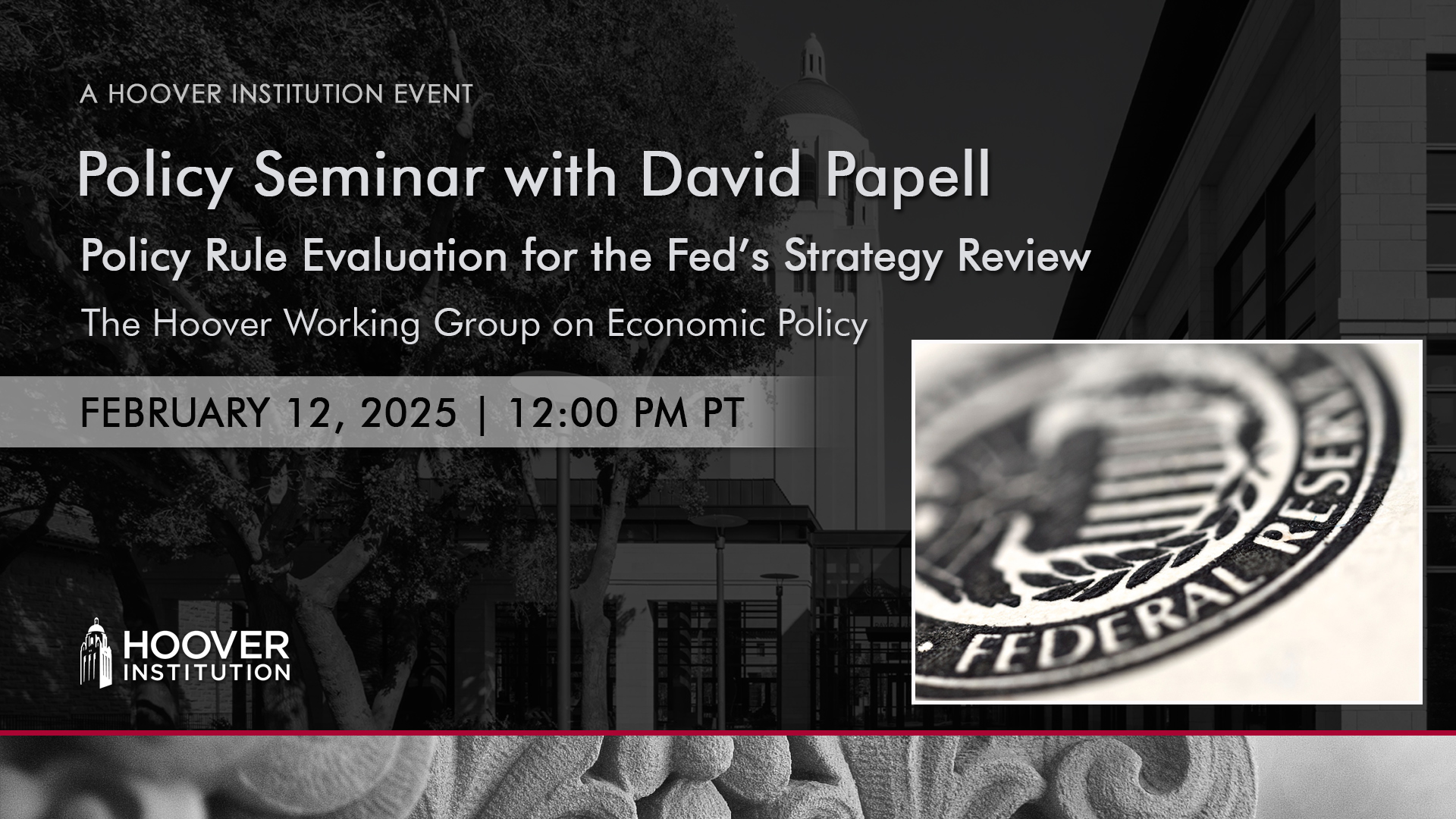
David Papell, Joel W. Sailors Endowed Professor of Economics at the University of Houston discussed “Policy Rule Evaluation for the Fed’s Strategy Review,” a paper joint with Sebin Nidhiri (University of Houston) and Swati Singh (University of Houston).
John Taylor, the Mary and Robert Raymond Professor of Economics at Stanford University and the George P. Shultz Senior Fellow in Economics at the Hoover Institution, was the moderator.
PAPER SUMMARY
The Federal Reserve Board started a strategy review at the beginning of 2025 and intends to complete by late summer of 2025. After its only previous review, the Federal Open Market Committee adopted a far-reaching Revised Statement on Longer-Run Goals and Monetary Policy Strategy in August 2020. We analyze and develop policy rules that are either in accord with the original 2012 statement or inspired by the revised 2020 statement and use the rules to evaluate monetary policy using the Federal Reserve Board/United States model. We evaluate policy rules categorized by traditional, shortfalls, Asymmetric Coefficient Inflation Targeting, and Asymmetric Target Inflation Targeting versions of non-inertial and inertial Taylor and balanced approach rules. Economic performance is better with balanced approach rules than with Taylor rules, worse with shortfalls rules than with traditional rules, better with inertial rules than with non-inertial rules, and better with the two asymmetric inflation targeting rules than with traditional rules.
To read the paper, click here
To read the slides, click here
WATCH THE SEMINAR
Topic: “Policy Rule Evaluation for the Fed’s Strategy Review”
Start Time: February 12, 2025, 12:00 PM PT
>> John Taylor: Very honored to have David Capell speak to us today, about a topic which is near and dear to many of our hearts. It's called Policy Rule Evaluation for the Fed's strategy review. And it goes into depth, more depth than you would like. I would like Sawat Singh, Swati Singh and David will lead us discussion right here, at this table.
So we're welcome, welcome back.
>> David Capell: Thank you so much, it's great. It's great to be.
>> John Taylor: Great to be here.
>> David Capell: Back, and actually with the Selma conference I get to come to Stanford three times in a year, which is as opposed to once, which is awesome.
>> John Taylor: So, people listening too?
>> David Capell: Yeah, why not, because I'm usually up there instead of here. And so, Sebin and Swati are fourth year PhD students at Houston who will answer all of your technical questions about the Lindbergh or Fervis models. So, Federal Reserve as everybody knows has started a strategy review, its second strategy review.
This has been, this was discussed at the January 2025 recent FOMC meeting, there's something in it. In the February 2025 Monetary Policy Report, there were press releases of earlier speeches by Chair Powell. I think the first was actually at Stanford where he meant where he mentioned it and that the new thing from the FOMC meeting is that it's scheduled to be completed in late summer 2025 where earlier they were talking about end of 2025.
Which of course he didn't say, I'm assuming would be announced at the Jackson Hole conference. Now, the history of this is that the first statement of longer run goals in monetary policy strategy in January 2012 made the 2% inflation target official and mitigated deviations of inflation from its longer run goal to employment from maximum employment.
Let me stop, I'm happy to take questions at any time, I don't need to wait for 45 minutes. So, the revised statement on long run goals monetary policy strategy August 2020 had the famous, or infamous flexible average inflation targeting, or fate where the quote is well known. The important thing, one important thing with this, is that it left persistently below likely aim moderately above, and some time undefined.
>> David Capell: defined. And the other half is the shortfalls mitigating shortfalls rather than deviations of employment from its maximum level. If you take maximum level as equivalent to the natural rate of unemployment, which is how Rich Clariter would describe it, it means that it reflects the flat Phillips curve that no longer raised the federal funds rate of unemployment is less than you star.
So, the strategy review was very heavily influenced by the experience during and mostly following the Great Recession between 2009 and 2019, and you had the first half with effective lower bound and then the second half with inflation, or the whole time with inflation under 2%. To the extent that John Williams made a very famous comment near the end of this that low inflation is our problem now, which, believe it or not, didn't quite work.
>> Speaker 4: But watch out, what you wish for, you might get it.
>> David Capell: What's that?
>> Speaker 4: What you wish for?
>> David Capell: True and so, but I think it's also worth to think that even though the review was released in August 2020, it was completed by the end of December 2019 and if it wasn't for COVID-19 would have been released early, early in 2020.
So it did not reflect COVID-19 in the slightest, it was very much the decade before. And the same time that the Jackson Hole conference and Chair Powell's speech was released, the Fed released a bunch of 8 maybe of papers that had been prepared for the strategy review. The one that's most relevant for purposes is one by Jonas Arias et al.of 8 these were all mixed between people from the board, people from regional Feds.
They were very high profile internal papers, and that paper in particular focused entirely on policy rules and alternative policy rules, and they focused on two things. One is average, or asymmetric average inflation targeting, where average you target the average inflation for whatever number of years before they used 8.
And the asymmetric is that you do that if inflation's below 2%, but you don't do that from to try to go down. And the idea is you're trying to stimulate the economy when inflation is below 2% more than a traditional tailor bounce approach rules. They also make up strategies for Federal Funds Rate 1/2 Federal Funds Rate, which are makeup strategies, and these make up strategies focused on the same idea except length of time at the effect of lower bound, John?
>> John Cochrane: So this whole question of promises about the future are going to stimulate today. There's two distinct categories of model behind this. One is the traditional adaptive expectations Old Keynesian view, which is basically, just we're going to talk down the long end of the yield curve. Essentially, we're promising lower interest rates out in the future.
That'll talk down long yields today long yields go down, that helps. The other is, I'll call it New Keynesian magic about equilibrium selection by promises out in the future. And the farther out you make the promise, the more effective it is today. And I'm sure you're familiar to what extent are these Fed internal studies taking one versus the other view.
Did the Fed even talk about Talk about how do we think this works. How much of it was infected by, well, Mike Woodford's famous Jackson Hole's speech, which was entirely this new Keynesian magic.
>> David Capell: I think for the Fed strategy review as opposed to the whole compass of Fed stuff.
Right, or the Fed right for that V or speeches, things like that associated at the time. The real focus is on these policy rules and I don't think there really was much discussion of which old Keynesian or New Keynesian model.
>> John Cochrane: Why did they say this was going to work to stimulate today?
>> David Capell: Going to tell you that in a minute.
>> John Cochrane: All right,
>> David Capell: so maybe two minutes. Now the principles for the 2019 review, these are articulated by Rich Clarida in 2022, but basically starting from, basically September from 2020 in a series of speeches, at least one or one here.
And one principle is asymmetric, that you want to raise inflation moderately above whatever that is, 2% from below, but you don't want to lower inflation below 2% from above. Second, it's time consistent. And time consistent is why at least in my mind, the Fed did not adapt, adopt average inflation or asymmetric average inflation or make up or make up rules.
And he famously described fate here, I believe as ex ante and consistent and export and ex post consistent. And let's not talk about that, that we could leave that aside. So but let's look, let's go to now 2025 strategy review. So reasonable to assume that the next 5 or 10 years would be like the previous 5 or 10 years.
That doesn't, always doesn't, it never works. But it's the best sort of like a unit route. The best you can do is the current situation. So what do we have now? Cycles of pandemic recovery, inflation disinflation, which hopefully won't be repeated and not a good basis for the review.
And quickly the experience following the COVID 19 recession, fate was completely irrelevant. Inflation went up. Annualized core PC inflation went up from 1.7% in March 2021 to 3.4% in June 2021. And even this is a paper that Ruxandra and I have that hasn't really seen the light of day yet.
If you just do a fate rule, it doesn't even help you then because the fate pushes you from further below the effective load bound to a little closer to the effect of load bound but still negative shortfalls. Unemployment wasn't above 4% to March of 2022 and just played no role there. So.
>> Speaker 4: It's 4.0 now.
>> David Capell: Yes, that's 4.0 now.
>> Speaker 4: Exactly.
>> David Capell: Exactly. Yes, it's really not over. Yes and so I think everybody, I think including myself, interprets statements by Chair Powell in the light of what they would like to see the Fed do. So I think but one is here is that we're not going to Fed's not going to stay with the 20191 but the Fed is concerned with the of having the effective lower bound hitting more often than in the pre 2008 past.
And that part of it is the fall perceived fall in our star which in the SEP has gone from 2 to 0.5 and now back up to 1 to 1. But 1 is still smaller than 2.
>> Speaker 5: With the inflation boat in 2021, did the Fed say well this is what we wanted, we wanted inflation to creep up above 2 or 3% and looked at faith.
That's exactly what we promised when they never so what's the reason why did they never say have a victory lap. And say look now we have high inflation compensating for lower inflation as before, just as promised?
>> David Capell: No, my interpretation of that is that and again I will take this from numbers which Clarida gave in this paper Vixandra.
And I published last fall on my interpretation is that moderately above was much closer to say 2.5, say not 3.5, 4 and certainly not 9. So they basically didn't have a chance to take a victory lap because they went from 1.7 to 3.5. So there was no opportunity.
>> John Cochrane: They were still saying well our forecasts say it'll go down to 2.5. So we're still within fate. Well they were in some sense even when inflation was well above 2, they were saying well our forecasts say this is all transitory and it'll go away in June of 2021 when it went from 1.7.
>> David Capell: The FOMC forecast for the end of the year was 3. So that's still not 2.5. And I think the more ambiguous part is do we go back to 2012. Going back to 2012 there which he sort of hinted in the last press conference that would violate the idea of being more worried about the effect of lower bound.
So in our case, since we're evaluating these things rather than in some sense advocating we're sidestepping some of this.
>> John Cochrane: Before you go into chime in consistency, John Steinson had a good observation in our last monetary policy conference. He said I read fate, but I always read that there was an implicit footnote saying, by the way, if inflation gets really out of hand, raise rates.
And being surprised that footnote wasn't there. I would think with the big sort of structural uncertainties ahead, are we gonna go back to the 1970s? Are we gonna be Argentina? Are we back to the zero boundaries? There would be some sort of here's how we're going to react to events, not just, we're going to readjust the coefficients on the fixed rule.
>> David Capell: In terms of coefficients, the Fed never. Adopted a fate rule, right? In the 2021 Monetary Policy Report, they have an algebraic shortfalls rule for good reason.
>> John Cochrane: We're gonna adjust the adjectives. So instead of saying, we're gonna take the fate rule and say instead of moderately, we're gonna say, well, substantially, I mean.
But instead, there's these big unknowns, we might be back to zero bound in QE, we might be into fighting Argentina, we have contingency plans.
>> David Capell: Your guess is as good as mine, my guess is that they're not gonna be that specific. They're not good, and certainly, the other guess is, they're not gonna adopt the rule.
So they're not gonna say here's-
>> John Cochrane: Adjectives.
>> David Capell: They're not gonna say. And I'm not going to predict the adjectives. What we're going to do here is sort of talk about rules to try to satisfy some of these things. But the 90 and uncertainty is not something that rules are gonna help us with.
So I wanna talk a little bit about time inconsistency. So if we start with time inconsistent policies, Kydland, Prescott, 77, Calvo, 78, optimal control exercise, and we all know incentives of future governments to modify policies that are optimal in today's perspective. This is understood by rational agents, and you can improve with policy rules.
And if you want to go back to how you can do this and whether it's possible or not, I suggest reading Guillermo Calvo's 78 Econometrica and John Taylor's 79 Econometrica for a very diametrically opposed views of how the Fed could do that. You were more optimistic with Guillermo's work.
And I think your offices were on the same or different floors.
>> Speaker 6: At Colombia.
>> David Capell: At Colombia, yes, yes. And the policy rules that were assumed to be time consistent, this is not what the Fed background papers mean by time inconsistency. They mean time inconsistent rules. And so if we're looking at these rules, average inflation targeting rules, the T average, exactly what John just said, I really don't need to talk more about that.
You're going from below 2%, you get above 2%, the average thing says, or asymmetric average, I keep on calling it asymptotic average, asymmetric average tells you, you should stimulate the economy even though inflation's above 2%. That's not what you want to do, nobody's gonna believe you. That's the rule story.
And they do talk. It's not like these people writing these background papers didn't know about time inconsistency. They do talk about this, but in the two papers that just we'll focus on the one, what did they talk about? They talked about the solutions for time inconsistent policies. Reputation, Barro and Gordon, Patent Law in John's to the sort of general belief of the importance the Fed would solve this in your 79 paper.
But these are all applicable to time inconsistent policies, not time inconsistent rules. So we are not going to analyze time inconsistent policies, sorry, time inconsistent rules in this paper. And if you do, yeah, just like you had in 2019, you can do better, that, if you really believe, if you believe.
There just isn't any reason to believe that. Okay so principles for you. Okay, so your reviews, your rules can be symmetric or asymmetric. Symmetric would mean equally stimulative when inflation's under 2%, then restrictive, when inflation is above 2%. Traditional Taylor and balanced approach rules satisfy this, the 2012 statement satisfies this.
Asymmetric, more stimulative when inflation's below 2%, then restrictive when inflation is above 2%. And I will show you two proposed rules that, in mind, satisfies, the asymmetric satisfies the focus on the effect of lower bound but are time consistent. Listen, that's really, if you wanna ask, what is your one takeaway from the paper, is that that's what we do.
So there's no incentive to renege when you get above 2%. So this interpretation, I'll call it similar but it's not identical to Rich Clarida's. Okay, so the paper, we analyze Taylor-type policy rules with sort of the structure of the inflation gap and the output gap but not all the other stuff that people talk about, Taylor and balance approach.
We also talk about shortfall policy rules since February 2021. Mike Kiley has a recent paper that analyzes the shortfalls rules and finds that they don't work particularly well. We're gonna basically find the same things, not gonna emphasize that too much. And we have two proposed rules, the asymmetric coefficient inflation targeting rule, or ACIT, and the asymmetric target inflation targeting rule, or ATIT.
And so what do we do? We used the linearized version, or LINVER, of the FRB/US. FRB/US model is the main policy model. It's the model that the Fed staff uses in each Hill book to do their calculations and simulations. This's been available, sorry, 96, it's been available since, I think, 2014 or something publicly, available.
Now, LINVER apparently, though I knew this, has existed about as long as FRB/US has. But they made no mention of this until 2022, where they released a working paper by David Reifschneider and Flint Brayton and basically documentation and code and how you could use this. The big advantage of LINVER Is that as long as you have it's linear or slightly nonlinear, it takes way less time to run the simulations we will show you each of them take about 30 minutes on a run of the mill.
PC Furbus is like a whole different world. And ex post we've learned that lots of power papers evaluating policy rules that said they were furbus were actually L going back to Weifschneider and Williams papers by Bernanke, Kylie and Roberts. All of these papers used LINVER. They said Ferbus because LINVER wasn't available.
So what do we do? We evaluate rules by quadratic loss functions. A whole lot of different ones. Inflation gaps, output gaps with and without the change in the federal funds rate. Sorry. It should be symmetric and shortfalls, not symmetric and asymmetric. I'm trying not to use asymmetric to mean two different things in the paper.
So symmetric and shortfalls. And on expectations that we have for the expectations financial market participants and wage and price setters have model consistent expectations. Other agents or rational expectations, other agents have VAR or adaptive expectations. She'll be first. Forgive me a second and basically you've a bunch of choices here.
You can have all agents having model consistent expectations. You could just financial market participants, but the others not. Not choices. It's what we do is it's robust to any of these and we don't talk about it in the paper except for having all agents having VAR expectations. And I thinking that financial market participants, or even now wage and price setters have adaptive expectations goes against about 50 years of macroeconomics.
So you first.
>> Speaker 7: I just wanted to ask if anybody is considering deviation in the sense of actually having the price level or price level path. And an argument I made at Brookings last fall is that what we're seeing is that an economy where they were at or below the 2% inflation target for a long time.
Many, many contracts are not indexed, even long term contracts and therefore that price path can really matter. And we're seeing all these other costs of inflation that we haven't put in our model like Eric Hearst's paper. And I certainly saw it being on the University of California Task Force for Investment Retirement because that generous pension, it turns out fully indexes up to 2% and nothing between 2 and 4%.
And they never tell their employees the effects of compound inflation. So it struck me, given that people in this kind of economy actually care about the price level as well, seems like they should be targeting the price path. It could have a slope of 2% kind of thing and that you just try to keep it there.
Otherwise we have this hysteresis where this transitory inflation consumers suddenly realize my goodness. Transitory inflation means permanent price changes and that can have effects on a lot of people.
>> David Capell: I think my answer is that I'm not saying it's not an interesting thing to do or to think about or write papers about.
It's not what we've done. There are lots of stuff. One thing by the way should have mentioned with the LINVER model there's no reason to think these results are going to hold across other models. No reason whatsoever. And in fact one very specific thing between Taylor and balanced approach rules in fact we talked about when we talked about your paper with Volkerwil.
And back in 2009 is that you get different results with lower loss with balanced approach than the Taylor rules for the Ferbus model. But not for the Smets and Bouder or Klestian, Weichenbaum and Evans model. So I'm just the defense I'm gonna give for this is that we vote the title for reason and evaluation for the Fed strategy review.
The main part of what the Fed and the Fed does have they have do have the SG models things but in terms of the policy part. No reason to believe that the main focus isn't going to be on the Ferberus or the Linver model as opposed to other models but I came no claim for.
>> Speaker 5: But if I may follow up, price pass targeting seems to be the logical solution if you have undershooting of inflation for a while how do you formulate the overshooting. How long should it last if you have a price pass in mind and some kind of rule how fast you get to that that's a nice time consist policy that could be formulated.
I wonder why the Fed never never went there. Do you know.
>> David Capell: I have or nominal GDP.
>> Speaker 5: Nominal GDP targeting would be another one is another one and I guess what now what I will say is that the LINVER model the FERP model is very constrained on what you can do.
And we've pushed the boundaries of the constraint beyond what anyone of the Fed has done but we've run up against other boundaries on it. And I have no idea and seven or SWATI could probably answer that question better than me whether anything that would even be feasible in the context of that model.
>> John Cochrane: Let me also push because this is also important in Europe too. Another way of phrasing it is do we measure our 2% inflation target as entirely forward looking with bygones or bygones. Or do we say over a period of five years we want to average 2% inflation, which means if you're above 2% you got to have some below 2%.
That's another even easier way. You don't have to say pros level target people are nuts. You just have to how do we interpret 2% average inflation?
>> Speaker 5: You're going to be below 2% for two years and then you have to go.
>> John Cochrane: Well that's just, it's another. And the reason I think.
>> David Capell: I'm gonna stop the reason this is a really interesting. But I'm never gonna get to my results if we spend the entire time.
>> John Cochrane: I do have an actual question. This is actually a question model you're using. New Keynesian or Old Keynesian, by which I mean.
>> David Capell: You actually asked me that before.
>> John Cochrane: Stability conditions is the table rule giving you determinacy or stability?
>> David Capell: The Phillips has this, these forward looking aspects and backward looking aspects. So from my looking at it, I really don't know whether you're talking about determinacy or stability there because there's all this, there's all this stuff.
>> John Cochrane: Well, we can find out. This is easy. Set an interest rate peg. What happens? Does the model have multiple solutions? Does it say I can. I can't solve with this, because it violates conditions, or is it stable and comes back?
>> David Capell: I'm not sure if that's within the context of the model.
So, if you want to say just the Phillips curve, okay, whether it's an old Keynes, you know, I mean, it's a mix of the two.
>> John Cochrane: No, this is a property of the entire model. What are the eigenvalues?
>> David Capell: I would be very doubtful that you could actually ask that question of, within the context of the, of the model.
It's an interesting question, but as I said there's a lot of things you cannot, there's very little that you can do within them.
>> John Cochrane: You can set Taylor rule coefficients to zero, and see what happens. So if the Taylor rule, if it's I equals peg, you can do that, what happens?
Because this is really crucial to what are we telling the Fed? That you have to select multiple equilibria correctly? Are we telling the Fed you got to bring inflation back faster?
>> David Capell: I need to think about that, I'm not. Yeah, let me just leave it as it's an interesting thing to think about and leave it there.
>> John Cochrane: But I asked Ben Bernanke this question, and he didn't know, then I could be in good company.
>> John Cochrane: Simple question.
>> David Capell: So, traditional policy rules. Okay, you all know what a non inertial Taylor rule is. R is the nominal federal funds rate. Uppercase, lowercase, R star is the neutral real interest rate inflation.
PI star is always going to be 2 and the Y is output gap, right? So, that's a traditional tailor.
>> Speaker 8: Does Lindver have a constant R star?
>> David Capell: Yeah, Lindver has a constant R star, which you, which we'll set it at. We said it here is 0.9 to 2.
Because my sense is that, you know, R star has been drifting over time, you know, drifted way down, you know, may have come back, you know, and how, and I think that's one of the reasons that the Fed doesn't like models.
>> Speaker 8: You know, they like models for, you know, like, well, this is what the model would be, but in the real world, our star is actually different.
So, we're going to like shade ourselves down from, you know, give some reasons to play around. And if you're evaluating something that's not consistent with the real world, you're only finding good results for a model, you're not finding good results for, you know, the way the world actually works.
And so, we're saying at any in time would type, and this is as the effect of lower bound, the R star influences how often the effect of lower bound binds in the model. And so the optimal policy could be very different in a world where R star is fluctuating.
So you could do these types of simulations, putting in some drifts in R star, see how that affects. Absolutely, again, I'm going back on my fallback position of evaluating rules for the Fed strategy review. What's the R star? The R star is whatever it is currently. So, if we were writing this paper today instead of the last version a month ago or two months ago, we would have one instead of 29.
That's not going to make a lot of difference.
>> Speaker 4: And let's think about Ustar. U star is substantial.
>> Speaker 6: Exactly.
>> David Capell: Yeah, now remember, the answer to that is that we're looking at policy rules with Y instead of with U. Although, we're going to look at loss functions, but we are going to look at loss functions view.
And that's actually internal to the model.
>> Speaker 4: Well, you can map U star into
>> David Capell: if you know what Okun's Local efficient is. And since, I think I've read everything you've ever written about, we know that's changed also, but maybe not recently, okay?
>> John Cochrane: Important rules of the game that you're setting here, which encompasses all of these.
You're not allowing the Fed to respond to shocks, right? Because in any new Keynesian model, the optimal policy rule responds to shocks and sets inflation exactly equal to target every period. So, you're not asking what's the optimal policy rule in Linver which you could ask, and you're really importantly saying and by the way, you're not allowed to respond to shocks.
>> David Capell: But here you have a fixed policy rule, and you're simulating a basis based on shocks, and I'm going to move forward. So, the inertial, because I think I was told that I should stop talking, and ask for questions by at 1 o'clock so I may cut questions.
I think I'll cut your questions off now. No, so you could have an inertial Taylor rule where you get part of the way the standard one is the 0.85 and 0.15. You can have a non-inertial balanced approach rule where you double the coefficient on the output gap, inertial balanced approach rule shortfalls rules.
We take a non-inertial shortfall rule on the inflation side, it's the same as the Taylor rule on the output gap side. It is that if GDP is below potential GDP, or unemployment is above U star, then you do what you did before, and you stimulate it. But if unemployment's below you start, or GDP is above, you don't raise the interest rate for that reason.
>> John Cochrane: What do you do about the zero bound? When the rule hits zero bound?
>> David Capell: We will have results that where you can't go below the effective lower bound. And that's all really what I'm going to talk about today with results where you can go below the effective lower bound.
If you can go below the effective lower bound, you can interpret this as. Since you only do it with quantitative easing, then think of that as a sort of shadow, as a sort of shadow rate for that. And I'm going to say I'll present no numbers with that, it's all in the paper.
I'll say one thing about it later, then you have the other types of rules. Okay, so what do we do? We have one, as we call the asymmetric coefficient inflation targeting. The idea of the asymmetric coefficient targeting is that on the top line there, if inflation is greater than 2, okay, then you follow the Taylor rule, or the balance approach rule or whatever version of that.
If inflation is less than 2, then you raise the coefficient on the inflation gap, the inflation gap is negative. You raise the coefficient, you stimulate more. So, the key here is that you're stimulating the economy more when inflation is less than 2%, but as soon as inflation exceeds 2%, you stop doing that and you flip.
To the Taylor rule and that's why this is time consistent because you are not stimulating the economy when inflation is above 2% there's no moderately above. And that's why, because you can say you're going to do this and then you can do this and you're not reneging on anything.
We do three coefficients 1, 1.5 and 2 for that. Obviously you want something it has to be bigger than 0.5. It's arbitrary. I'll talk a little bit about what happens when you get high asymmetric target inflation targeting Remember the first thing that the Fed announced with the 2019 and the first thing they announced now is they are not raising the inflation target above 2%.
What we're talking about here is that if inflation is above 2% you have the traditional target. If inflation is below 2% then you have a bigger target. You have a bigger target because that gives you a more negative thing then for the same 0.5 coefficient you have more stimulus policy.
>> Speaker 5: And we would imply a jump in Rt just as you cross pi star like a minute. I guess everyone is-
>> David Capell: Because the gap is minuscule there's no jump.
>> Speaker 5: No. If you cross from above pi star to just below pi star, I mean, this is not a continuous function pi t-
>> David Capell: But if you go from 2.0 to 1.99 you can multiply it by a bigger number, you're not gonna get a discernible gap.
>> Speaker 5: No, I mean merging the pi cap T I mean just for the sake of the argument is thousand, right? Then he would suddenly go from Rt, at pi star you're exactly where you wanna be.
And then if pi t is 1.99 out of a sudden you're gonna lower interest rates dramatically.
>> David Capell: Yes. And that goes back to the argument of not in this context at all that there's a preference for very large coefficients even in the Taylor rule type of thing, infinite coefficient.
Because if you have an infinite coefficient you never violate it. That's why these loss functions were developed that have the change in the federal funds rate is to prevent is to penalize having these really big coefficients. In this case, when you respect the effect of lower bound it doesn't make much difference because you're talking about small things under there.
But in the version of the model where you can be under the effect of lower bound then it does matter and there is actually something in the paper could show. Brian we're not going there. But yes, that's done.
>> Speaker 5: What's more technical question whether we should be concerned about the policy rule.
What it says- Continues in the inflation.
>> David Capell: And so we do 2.5, 3, and 3.5. Again you can do different numbers but again I'm fairly sure if we had infinity then you would not do very well with the loss function when you don't impose the effect of lower bound and you don't have the penalty.
We're not that territory today. Okay, loss functions. Okay, we have symmetric loss functions. Loss function being the difference between inflation and target squared plus the output gap squared. And you could have which we call symmetric. Symmetric with the change in the federal funds rate we stick in the change in the federal funds rate squared that turns out to be not matter.
I'm not gonna talk about at all today. Shortfalls that if output is under y star, then you have the normal loss function. If output is greater than y star, you wipe out that output gap. Part of it that has the effect of having all of these shortfall loss functions giving you smaller loss than the.
Than the symmetric ones which is utterly irrelevant because you're just wiping out that part of it.
>> John Cochrane: You could do PT minus P star if you wanted to or you could do sum of PI T minus PI star over five years squared. I think we're all saying that this would be interesting.
>> David Capell: One it could be interesting. Whether it could be done in the constraints of the Linver model is something I don't know. But it's an interesting question to pursue. But I'm not going to talk about P today in my next 12 minutes.
>> John Cochrane: It's just a suggestion because even at the Fed they understand that people are mad about the price level.
So they are going to be thinking about this.
>> David Capell: Well, just look at the last election. No. Yeah, so I said I'm with you, I just don't know in this context if it could be done or not. That doesn't mean that we or somebody else do it in a different context who might be better suited to do it this.
But let's just hold off on that. I am now laying down the law. I'm not going to answer anything that has P in it. Okay, shortfalls and you can have it with the change. And we also substitute the unemployment gap in the loss functions for the output gap.
Okay, so we have eight types of rules, we have four versions of each rules, we have eight loss functions, we have policy rules with and without, the effect of lower bound, once we put in the with and without I think we're up to 512 in the paper. Okay I'm not gonna show you 512.
So here's what I'm gonna show you. We're basically gonna look at symmetric loss we're gonna do one thing with shortfalls but symmetric loss without the change in the federal funds rate putting that is irrelevant. So the first thing as we look at the Taylor rule, the balance approach rule, we look at non-inertial rules, inertial rules, and two takeaways from here one takeaway is that there are big differences between Taylor and balanced approach.
The losses with balanced approach rules are sort of smaller than the loss with Taylor rules that's why I think you should have just said that's That's just a form of the Taylor Rule in 2009, and gotten all the credit for it. Rather just call it the Taylor 1999 rule rather than the balanced approach rule, which by the way in the Fed stuff most of the time when they refer to Taylor rules, they're actually referring to balanced approach rules.
They sort of cut that, but the other part is inertial and non-inertial is very small differences here. Okay, now traditional, and shortfalls. So now, we're going to look at balanced approach inertial only because they were a little small, slightly smaller than the balance approach non-inertial does doesn't make any difference.
Their output gaps are now going to look with symmetric loss and shortfall loss. So basically, everything is going to be almost as the wisdom, right? So, let's look at two things. With traditional rules and shortfalls rules, and with symmetric loss, there was a huge difference between the traditional rules and shortfall rules.
The shortfall rules are a disaster on this, and this is something my colleague said in his 2024 paper. This is not original for us, but what happens when you do shortfalls loss? Well, the traditional rules still do better, but the gap is way smaller.
>> Speaker 5: Maybe, I'm missing something here, it says these are output gaps, but you're not optimizing giving the loss function, right?
So, I thought the rules are fixed in a fixed coefficient, and they would imply the same.
>> David Capell: We use the Lindver model, there's a Y star internal to the Linver model potential output. And so you get the output gap from.
>> Speaker 5: You get the output, I understand, you get the output gap.
So, if you put in a particular policy rule, you get a particular average output gap. But the loss function doesn't matter for getting the calculation for that output gap. But here it says something about loss function. Is, are these losses or are these the output gaps?
>> David Capell: These are losses.
>> Speaker 5: These are the losses.
>> David Capell: I'm sorry, the numbers are all, sorry, misinterpret what you said. The numbers are all losses, and they are losses.
>> Speaker 5: It was just thrown off by the title, output gap width.
>> David Capell: Yeah.
>> Speaker 5: You're using the output gap in the loss.
>> David Capell: We're using the output gap in the loss function with balance.
And by the way, we have the same things with the unemployment gap instead of the output gap. Nothing changes, I said. Basically, this is like six pages of tables, with picking out a few to show you. Okay, now what about the AC&C IT policy rule evaluation? So the first thing, is we're picking, taking the inflation gap coefficient of 1.5 to show here and again the coefficient itself.
These choice of coefficients is arbitrary, right? We're doing a range of coefficients, you could do other coefficients. But the point from this slide is very similar to the traditional rules. Bounce approach does much better than Taylor rules, and that non-inertial and inertial are tiny.
>> Speaker 8: David, what's happening to long rates in these models with non inertial rules?
Presumably they're much more volatile and that's going to mean much more risk in the banking system. That might, my understanding was that the whole emphasis on inertial rules is designed to protect the banking system to provide them a path that they can manage their longer term assets and engage in maturity transformation.
>> David Capell: See, I don't think any of that enters this model.
>> Speaker 8: No, nothing that doesn't enter, but that's distinct.
>> David Capell: My interpretation of the inertial rules comes, comes from the Fed wanting to smooth out, right?
>> Speaker 8: Why do they want to smooth? They want to smooth because the banking system, gets in trouble when interest rates are highly variable, patience part of their mission.
>> David Capell: I think wanting to smooth can be like, for example, Glenn Rudebush has a 96 paper on different ways of interpreting smoothing. And I don't think the word banking system appears, so I think the point can be more general. I'm not saying that it's not important with the banks, I think that the point could be more general than the bank system.
Okay, so now, let's look here at the, okay, differences between the traditional rules and the ACIT rule. Remember, the traditional rule has a coefficient of 0.5 on the inflation gap. I have three rules with the ACIT with 1, 1.5 and 2. So of course the traditional rule is the same loss, whatever you have with this, and again it's the same output gapsy metric, whatever, whatever and that the losses, the losses with the ACIT rules are uniformly under the losses with the traditional rules.
They're moderate, they're not as big as the losses with Taylor and Balanced approach, they're bigger than inertial, non-inertial. As the coefficient goes up, the difference increases at a decreasing rate. So you think that as you go hopefully you'd reach some sort of, you know, you're not, these differences are going up, but they're not, they're not as impossible.
They're not going to become in infinite, or this is as far as we've gone. Okay, the ATIT rules. Again, this is again with an inflation target. The asymmetric, the inflation target, not the inflation target of 3 Taylor balance approach. Again, what we've seen before, big differences there, small differences inertial and non-inertial.
And I think more interestingly is traditional and at IT policy rules with the different coefficients. Again, smaller with the ATIT rule than the traditional balanced approach rule moderate differences. Differences increase as you increase the inflation target when you're under 2%, but increase at a decreasing rate when you do that for the same increments.
There, one thing, we do this The only thing, yes?
>> John Cochrane: Since you're moving on to.
>> David Capell: What? Go ahead, yes?
>> John Cochrane: Not interesting to ask the optimal rule. So given a loss function, given a model, what's the optimal rule? Rather than I'm going to just try a bunch of different rules at it.
>> David Capell: As I said, I'm going to put that in the category of something that it might be interesting for somebody who finds that a more interesting question than I do to work on.
>> John Cochrane: Why didn't you find it an interesting question?
>> David Capell: Because I think that first of all, if you even go back to time inconsistency, all rules are suboptimal.
So now, you want to be talking about the optimal suboptimal rule. And I said I think that's a question that you could address, and people haven't addressed in smaller models, I don't think it's. Again, I keep on going back to this paper with the words in the title of Feds Strategy Review.
Now, you can expand past that and there's lots of other things, but,
>> John Cochrane: You will have to respond to referees who will ask this question. And I actually think it's an interesting answer, that you sort of trust this model well enough to evaluate how given rules work, but you don't trust it to calculate the optimal rule because you think that'll send it off into space somewhere.
Yeah, Tell the referees that.
>> David Capell: I should write that down, so that when you referee the paper, I know what the response would be.
>> Speaker 9: I'm going to ask a question on behalf of our audience today, okay? Because we have a lot of people here today, and I'm going to guess what one of their questions might be.
They have been schooled to think about the trade-off in terms of rules rather than discretion, okay? And now, we're thinking about a rule, and you know, an unsophisticated person might think these are all variations of a very similar rule, and yet they get very different loss functions, very different sort of results and answers.
How should they rethink what they have learned about the trade-off of rules rather than discretion?
>> David Capell: I mean, I guess I would call that what your audience has learned about rules versus discretion is really the 1970s time inconsistency. And again, for me, being a student of both John and Guillergia, it's sort of in my blood there, but this is in terms of different policy rules.
And I think here it's really a question of if you have a policy rule where, you know, which violates the time inconsistency, then you just can't even analyze it, and in fact, one sort of coda on that is within the Lina. You really can't analyze it because all model consistent expectations are assumed to be fulfilled, you know, again so?
>> Speaker 9: But for those of us who only came into this profession in a post rational expectations world, I would think they might be surprised how many things that look really similar to a Taylor rule at its face are so incredibly different in all different ways. And what they should take from that I think might be helpful.
>> David Capell: I think necessarily all that different. I think a lot of them very, you know, except for the tail, except for the Taylor balance approach that once, yeah, there are differences there, they're not big, they're moderate. And that seems a finding of people who look at those rules.
So, I mean maybe one way of saying, of saying that now I'm going to channel my inner John Taylor on this is that what's actually important is that you have a rule, and you follow the rule, and you establish that, and the secondary thing is which rule it is.
So you have to finish, hence rules rather than I have to finish. Okay, okay?
>> John Cochrane: So, one feature of all these things is that inflation neither spirals out of control if it turns out to an old Keynesian model, nor suffers multiple equilibrium volatility, it's a new Keynesian model.
Otherwise, a lot of the difference also then depends. In an old Keynesian model it's how quickly you get rid of inflation. In a new Keynesian model, all the details of the rules are an implicit time varying inflation target which you hit perfectly, and those are actually quite different.
>> David Capell: But again, as you know, the conditions for stability or determinacy are the same, it's the Taylor principle, right? Yes. In fact, we've had this discussion about sufficient. We're not going to go, okay?
>> John Cochrane: Why the model is giving different answers depends very much on whether what the model is doing is giving you determinacy about a time varying point, or is it giving stability, and then the question is how quickly does it come back?
So, the intuition.
>> David Capell: And I'll throw it back to you that I've believed your conclusion from your 2000, the 2010 or so JPE paper is that is, is that, is that there are all these issues with determinacy, but we shouldn't go back to non uniqueness. Let me take one minute and then open to questions.
Okay, what was that fair?
>> Speaker 6: The price level is the answer.
>> David Capell: All right, that was after 20,000. Okay, just really quickly one example of these are of course rules where you're not respecting the lower bound and just you have more stability more differences with these between the traditional rule.
If you look you know the biggest things just look at going down to like the 2011 Q1 that's the most dramatic thing that there's a pretty big difference in the prescription of these AT&T. Or ACIT rule than there is with the traditional these are, and this is with the Taylor rule balanced approach is a little smaller than that but we don't need to talk about that.
And you've seen the conclusions I will again say that my takeaway from this is basically you can do moderately better with our proposed rules than with the traditional rules. And not violate time inconsistency the way the average inflation targeting, or the makeup rules do, and so I'm now done.
So now, we can ask as many questions as you want.
>> John Cochrane: A short one it's an actual question.
>> David Capell: It could be long.
>> John Cochrane: This is a question mark with it, you didn't show much on the persistence and how quickly the RHO coefficients and your wonderful results from last.
Monetary policy conference, where if you have rho equals 1 and have a fully adjusting rule, then things get very different. So what about the optimal persistence? How quickly should you get back to the Taylor rule?
>> David Capell: Yeah, and you're right, we're looking at a different-
>> John Cochrane: So these were all persistence at 0
>> David Capell: Again, this is all model free, everything that it was presented before.
I mean, when you're talking about going back to the 2019 monetary policy.
>> John Cochrane: In here, I gather all of your rho's were 0-
>> David Capell: With rho's being-
>> John Cochrane: Rho is equal to- You have lagged interest rates, so you just-.
>> David Capell: No, no, no, we have inertial and non-inertial, we have 0 and 0.85.
>> John Cochrane: So quickly, how did inertial versus non-inertial work out?
>> David Capell: There's small differences.
>> John Cochrane: How about rho equals 1, what happens?
>> David Capell: Those are the only things that we've tried. Those are the leading candidates, right? But very little differences.
>> Speaker 6: I guess sort of getting back to Fed strategy review sort of question, I'm curious what your thoughts are around, I mean, what you think they're going to do.
And I mean my sense of things is the big question is whether they're going to kill faith or not. They're definitely going to keep inflation targeting. I interviewed a Fed governor last week. She said there's one thing, 2% inflation targeting is one that we should keep. But to me, I see this really more in the lens of, I guess, the sort of political, I guess, regret aversion sort of minimization challenge.
Which is that the Fed already has some egg on its face, even if they won't admit it, most won't admit it. And they haven't even got inflation back to 2% yet. And my sense of things, and correct me if I'm wrong, is that they probably would err on the side of not making changes to the mandate until they get at least inflation back to 2% first.
Maybe that would be a reason to keep FAIT, even though FAIT was something designed for the pre-COVID period. But again, I mean, maybe if they did that, they'd tailor FAIT to being more sort of universal than it was sort of before. But I'm curious what you think about this calculus around to keep it.
>> David Capell: The first thing is, the first thing they said is, we are not gonna change the 2% target. Or, as Rich Clarida said the last time, full stop. I'll say it again, we're not going to change the 2%. And they've said it again. So that's clearly off the table.
Now, I would be really, really, really surprised, a little less surprised than the last one, if they said, FAIT and shortfalls that we did in 2019 were great, we should keep them. I, I really don't see that now that, so I'd also be surprised, but less surprised if they, a little less surprised if they said let's just go back to 2012.
And the reason I'd be less surprised is two reasons. One, it doesn't go along with the worry about the effect of lower bound that Jay Powell emphasized a lot. And the other reason is that they're not going to say, we made a mistake in 2019, we're gonna go back into that.
They're not doing that, okay. So I think what they're gonna do is do something that's gonna somehow muddle their way through this. They will not say we're gonna have a policy rule, although I'd be surprised if they didn't have papers that looked at policy rules and that. I mean, I gave this paper in early December the board, and of course my suggestion was that they should like at least analyze R2 proposed rules.
And they didn't all say yes, we're going to do that and make it a focus of the review. But of course they also didn't say no. So of course, but what sort of thing they would come up with to replace, I think.
>> Speaker 8: So in a lot of Fed speak, there's emphasis on anchoring inflation expectations at the long term.
And they get forecasts from the blue chip forecasters, they get the forecast from the tips, treasury spread.
>> David Capell: They get everything.
>> Speaker 8: Yeah, and so they clearly look at those, and that goes into the discussions they have at the FOMC. Pi here, I take it, is actual inflation.
>> David Capell: Yes.
>> Speaker 8: What if you made it expected inflation, model consistent expected inflation as the driver of r* plus expected inflation.
>> David Capell: I think what was this model consistent inflation would be basically inflation from forecasts from a Phillips curve. And that goes against the flat Phillips curve, other stuff.
And in fact, like Rich Clarida, who, of course, is not there anymore, but he emphasized over and over again their interest looking at this index of common inflation expectations. Sort of looking at everything but the whole, not going to be looking to the forecasts from Phillips curves. And they could be back to that, but, I mean, I think the decade between 2019 wasn't kind to that internal argument with the Fed and the argument that we need to be looking at inflation forecasts, not inflation rates.
>> Speaker 5: So here's something that puzzles me about the numerical results that you showed before, which is you have a linear model, so let's say you have a symmetric loss function. Then intuition would suggest that a symmetric policy rule would do better than an asymmetric policy rule, right? Because you want to, everything is symmetric, so you want to do the same thing on both sides to minimize the loss, as it were.
But you showed results that look like the asymmetric rules did better. And I'm wondering whether that's about really getting closer to the optimum that John suggested. So let's say really what you ought to do is just being more aggressive on inflation. But now you're comparing two rules, one that is sort of somewhat soft on inflation to one that's more aggressive on one side of the inflation, so becoming more aggressive.
So it's not the asymmetry that does the trick, it's just really about the rule becoming more aggressive with inflation. And if that intuition is correct, that suggests that maybe the way you want to compare symmetric and asymmetric rules is, if you do little more on the one side, you should also do a little less on the other side.
So on average you're doing the same. It seems very puzzling to me that asymmetric policy rules should do better given the symmetry and the linearity of the model involved.
>> David Capell: And again, I mean, yes, we know that bigger inflation, bigger coefficients on inflation, will do better until they don't when you put in penalizing changes in the federal funds rate.
So what we're gonna, is say, okay, keep that 0.5 when you're above 2%. Because again, we could take what we had and say we made it to make it one of it's above in both rules, and then bigger ones under. But the reason that I think these asymmetric rules work somewhat better, not dramatically better, right?
But somewhat better, is that they push inflation closer to 2% from below, without getting you to point where you're getting into the-
>> Speaker 5: There's a question over here.
>> Speaker 10: This might be a bad question, but I'm wondering, for all these coefficients, why don't you just let them float and optimize over one of these loss functions?
Why 0.5 or 1.5? Why not just have them be variables and then optimize the loss functions for these things?
>> David Capell: Part of it is that goes as we're in the realm of what let's call simple policy rules, where you're saying, here's the coefficient, people know what the coefficient is.
And that helps with the policy, if you go into these time-varying coefficients, or each period, things like that, people just don't have an idea of what the policy is. And I think that's the argument for the simple rules, which, of course, are not optimal rules.
>> John Taylor: Thank you, David.
>> David Capell: Thank you.